SportFlow

SportFlow applies machine learning algorithms to predict game outcomes for matches in any team sport. We created binary features (for classification) to determine whether or not a team will win the game or even more importantly, cover the spread. We also try to predict whether or not a game’s total points will exceed the over/under.

Of course, there are practical matters to predicting a game’s outcome. The strength of supervised learning is to improve an algorithm’s performance with lots of data. While major-league baseball has a total of 2,430 games per year, pro football has only 256 games per year. College football and basketball are somewhere in the middle of this range.

The other complication is determining whether or not a model for one sport can be used for another. The advantage is that combining sports gives us more data. The disadvantage is that each sport has unique characteristics that could make a unified model infeasible. Still, we can combine the game data to test an overall model.

Data Sources

SportFlow starts with minimal game data (lines and scores) and expands these data into temporal features such as runs and streaks for all of the features. Currently, we do not incorporate player data or other external factors, but there are some excellent open-source packages such as BurntSushi’s nflgame Python code. For its initial version, SportFlow game data must be in the format below:

NCAA Basketball Data
season	date	away.team	away.score	home.team	home.score	line	over_under
2015	2015-11-13	COLO	62	ISU	68	-10	151
2015	2015-11-13	SDAK	69	WRST	77	-6.5	136
2015	2015-11-13	WAG	57	SJU	66	-5.5	142
2015	2015-11-13	JVST	83	CMU	89	-18	142.5
2015	2015-11-13	NIAG	50	ODU	67	-18	132
2015	2015-11-13	ALBY	65	UK	78	-20	132.5
2015	2015-11-13	TEM	67	UNC	91	-9.5	145
2015	2015-11-13	NKU	61	WVU	107	-23.5	147.5
2015	2015-11-13	SIE	74	DUKE	92	-24	155
2015	2015-11-13	WCU	72	CIN	97	-20	132
2015	2015-11-13	MSM	56	MD	80	-21.5	140
2015	2015-11-13	CHAT	92	UGA	90	-10.5	136
2015	2015-11-13	SEMO	53	DAY	84	-19	140
2015	2015-11-13	DART	67	HALL	84	-11	136
2015	2015-11-13	CAN	85	HOF	96	-10.5	150.5
2015	2015-11-13	JMU	87	RICH	75	-9	137.5
2015	2015-11-13	EIU	49	IND	88	-25	150
2015	2015-11-13	FAU	55	MSU	82	-23.5	141
2015	2015-11-13	SAM	45	LOU	86	-23	142
2015	2015-11-13	MIOH	72	XAV	81	-15.5	144.5
2015	2015-11-13	PRIN	64	RID	56	1	137
2015	2015-11-13	IUPU	72	INST	70	-8	135.5
2015	2015-11-13	SAC	66	ASU	63	-18	144
2015	2015-11-13	AFA	75	SIU	77	-5.5	131
2015	2015-11-13	UNCO	72	KU	109	-29	147.5
2015	2015-11-13	BALL	53	BRAD	54	3	135
2015	2015-11-13	USD	45	USC	83	-12.5	140
2015	2015-11-13	UTM	57	OKST	91	-12	141.5
2015	2015-11-13	COR	81	GT	116	-17	130
2015	2015-11-13	MOST	65	ORU	80	-4.5	133.5
2015	2015-11-13	DREX	81	JOES	82	-9.5	127.5
2015	2015-11-13	WMRY	85	NCST	68	-12.5	149
2015	2015-11-13	SF	78	UIC	75	1.5	148.5
2015	2015-11-13	PEAY	41	VAN	80	-24.5	144
2015	2015-11-13	CSN	71	NIU	83	-9.5	134.5
2015	2015-11-13	UCSB	60	OMA	59	-2.5	157.5
2015	2015-11-13	UTSA	64	LOYI	76	-14	138.5
2015	2015-11-13	BRWN	65	SPU	77	-2	130.5
2015	2015-11-13	NAU	70	WSU	82	-10.5	145

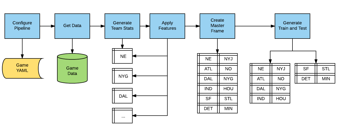
The SportFlow logic is split-apply-combine, as the data are first split along team lines, then team statistics are calculated and applied, and finally the team data are inserted into the overall model frame.

Domain Configuration

The SportFlow configuration file is minimal. You can simulate random scoring to compare with a real model. Further, you can experiment with the rolling window for run and streak calculations.

sport.yml

sport:
    points_max      : 100
    points_min      : 50
    random_scoring  : False
    seasons         : []
    rolling_window  : 3

points_max:: Maximum number of simulated points to assign to any single team.
points_min:: Minimum number of simulated points to assign to any single team.
random_scoring:: If True, assign random point values to games [Default: False].
seasons:: The yearly list of seasons to evaluate.
rolling_window:: The period over which streaks are calculated.

Model Configuration

SportFlow runs on top of AlphaPy, so the model.yml file has the same format.

model.yml

project:
    directory         : .
    file_extension    : csv
    submission_file   : 
    submit_probas     : False

data:
    drop              : ['Unnamed: 0', 'index', 'season', 'date', 'home.team', 'away.team',
                         'home.score', 'away.score', 'total_points', 'point_margin_game',
                         'won_on_points', 'lost_on_points', 'cover_margin_game',
                         'lost_on_spread', 'overunder_margin', 'over', 'under']
    features          : '*'
    sampling          :
        option        : False
        method        : under_random
        ratio         : 0.0
    sentinel          : -1
    separator         : ','
    shuffle           : False
    split             : 0.4
    target            : won_on_spread
    target_value      : True

model:
    algorithms        : ['RF', 'XGB']
    balance_classes   : False
    calibration       :
        option        : False
        type          : isotonic
    cv_folds          : 3
    estimators        : 201
    feature_selection :
        option        : False
        percentage    : 50
        uni_grid      : [5, 10, 15, 20, 25]
        score_func    : f_classif
    grid_search       :
        option        : True
        iterations    : 50
        random        : True
        subsample     : False
        sampling_pct  : 0.25
    pvalue_level      : 0.01
    rfe               :
        option        : True
        step          : 5
    scoring_function  : 'roc_auc'
    type              : classification

features:
    clustering        :
        option        : False
        increment     : 3
        maximum       : 30
        minimum       : 3
    counts            :
        option        : False
    encoding          :
        rounding      : 3
        type          : factorize
    factors           : ['line', 'delta.wins', 'delta.losses', 'delta.ties',
                         'delta.point_win_streak', 'delta.point_loss_streak',
                         'delta.cover_win_streak', 'delta.cover_loss_streak',
                         'delta.over_streak', 'delta.under_streak']
    interactions      :
        option        : True
        poly_degree   : 2
        sampling_pct  : 5
    isomap            :
        option        : False
        components    : 2
        neighbors     : 5
    logtransform      :
        option        : False
    numpy             :
        option        : False
    pca               :
        option        : False
        increment     : 3
        maximum       : 15
        minimum       : 3
        whiten        : False
    scaling           :
        option        : True
        type          : standard
    scipy             :
        option        : False
    text              :
        ngrams        : 1
        vectorize     : False
    tsne              :
        option        : False
        components    : 2
        learning_rate : 1000.0
        perplexity    : 30.0
    variance          :
        option        : True
        threshold     : 0.1

pipeline:
    number_jobs       : -1
    seed              : 13201
    verbosity         : 0

plots:
    calibration       : True
    confusion_matrix  : True
    importances       : True
    learning_curve    : True
    roc_curve         : True

xgboost:
    stopping_rounds   : 30

Creating the Model

First, change the directory to your project location, where you have already followed the Project Structure specifications:

cd path/to/project

Run this command to train a model:

sflow

Usage:

sflow [--train | --predict] [--tdate yyyy-mm-dd] [--pdate yyyy-mm-dd]

--train: Train a new model and make predictions (Default)
--predict: Make predictions from a saved model
--tdate: The training date in format YYYY-MM-DD (Default: Earliest Date in the Data)
--pdate: The prediction date in format YYYY-MM-DD (Default: Today’s Date)

Running the Model

In the project location, run sflow with the predict flag. SportFlow will automatically create the predict.csv file using the pdate option:

sflow --predict [--pdate yyyy-mm-dd]