NCAA Basketball Tutorial

SportFlow Running Time: Approximately 15 minutes

In this tutorial, we use machine learning to predict whether or not an NCAA Men’s Basketball team will cover the spread. The spread is set by Las Vegas bookmakers to balance the betting; it is a way of giving points to the underdog to encourage bets on both sides.

SportFlow starts with the basic data and derives time series features based on streaks and runs (not the baseball runs). In the table below, the game data includes both line and over_under information consolidated from various sports Web sites. For example, a line of -9 means the home team is favored by 9 points. A line of +3 means the away team is favored by 3 points; the line is always relative to the home team. An over_under is the predicted total score for the game, with a bet being placed on whether not the final total will be under or over that amount.

NCAA Basketball Data
season	date	away.team	away.score	home.team	home.score	line	over_under
2015	2015-11-13	COLO	62	ISU	68	-10	151
2015	2015-11-13	SDAK	69	WRST	77	-6.5	136
2015	2015-11-13	WAG	57	SJU	66	-5.5	142
2015	2015-11-13	JVST	83	CMU	89	-18	142.5
2015	2015-11-13	NIAG	50	ODU	67	-18	132
2015	2015-11-13	ALBY	65	UK	78	-20	132.5
2015	2015-11-13	TEM	67	UNC	91	-9.5	145
2015	2015-11-13	NKU	61	WVU	107	-23.5	147.5
2015	2015-11-13	SIE	74	DUKE	92	-24	155
2015	2015-11-13	WCU	72	CIN	97	-20	132
2015	2015-11-13	MSM	56	MD	80	-21.5	140
2015	2015-11-13	CHAT	92	UGA	90	-10.5	136
2015	2015-11-13	SEMO	53	DAY	84	-19	140
2015	2015-11-13	DART	67	HALL	84	-11	136
2015	2015-11-13	CAN	85	HOF	96	-10.5	150.5
2015	2015-11-13	JMU	87	RICH	75	-9	137.5
2015	2015-11-13	EIU	49	IND	88	-25	150
2015	2015-11-13	FAU	55	MSU	82	-23.5	141
2015	2015-11-13	SAM	45	LOU	86	-23	142
2015	2015-11-13	MIOH	72	XAV	81	-15.5	144.5
2015	2015-11-13	PRIN	64	RID	56	1	137
2015	2015-11-13	IUPU	72	INST	70	-8	135.5
2015	2015-11-13	SAC	66	ASU	63	-18	144
2015	2015-11-13	AFA	75	SIU	77	-5.5	131
2015	2015-11-13	UNCO	72	KU	109	-29	147.5
2015	2015-11-13	BALL	53	BRAD	54	3	135
2015	2015-11-13	USD	45	USC	83	-12.5	140
2015	2015-11-13	UTM	57	OKST	91	-12	141.5
2015	2015-11-13	COR	81	GT	116	-17	130
2015	2015-11-13	MOST	65	ORU	80	-4.5	133.5
2015	2015-11-13	DREX	81	JOES	82	-9.5	127.5
2015	2015-11-13	WMRY	85	NCST	68	-12.5	149
2015	2015-11-13	SF	78	UIC	75	1.5	148.5
2015	2015-11-13	PEAY	41	VAN	80	-24.5	144
2015	2015-11-13	CSN	71	NIU	83	-9.5	134.5
2015	2015-11-13	UCSB	60	OMA	59	-2.5	157.5
2015	2015-11-13	UTSA	64	LOYI	76	-14	138.5
2015	2015-11-13	BRWN	65	SPU	77	-2	130.5
2015	2015-11-13	NAU	70	WSU	82	-10.5	145

Step 1: First, from the examples directory, change your directory:

cd NCAAB

Before running SportFlow, let’s briefly review the configuration files in the config directory:

sport.yml:: The SportFlow configuration file
model.yml:: The AlphaPy configuration file

In sport.yml, the first three items are used for random_scoring, which we will not be doing here. By default, we will create a model based on all seasons and calculate short-term streaks of 3 with the rolling_window.

sport.yml

sport:
    league          : NCAAB
    points_max      : 100
    points_min      : 50
    random_scoring  : False
    seasons         : []
    rolling_window  : 3

In each of the tutorials, we experiment with different options in model.yml to run AlphaPy. Here, we will run a random forest classifier with Recursive Feature Elimination and Cross-Validation (RFECV), and then an XGBoost classifier. We will also perform a random grid search, which increases the total running time to approximately 15 minutes. You can get in some two-ball dribbling while waiting for SportFlow to finish.

In the features section, we identify the factors generated by SportFlow. For example, we want to treat the various streaks as factors. Other options are interactions, standard scaling, and a threshold for removing low-variance features.

Our target variable is won_on_spread, a Boolean indicator of whether or not the home team covered the spread. This is what we are trying to predict.

model.yml

project:
    directory         : .
    file_extension    : csv
    submission_file   : 
    submit_probas     : False

data:
    drop              : ['Unnamed: 0', 'index', 'season', 'date', 'home.team', 'away.team',
                         'home.score', 'away.score', 'total_points', 'point_margin_game',
                         'won_on_points', 'lost_on_points', 'cover_margin_game',
                         'lost_on_spread', 'overunder_margin', 'over', 'under']
    features          : '*'
    sampling          :
        option        : False
        method        : under_random
        ratio         : 0.0
    sentinel          : -1
    separator         : ','
    shuffle           : False
    split             : 0.4
    target            : won_on_spread
    target_value      : True

model:
    algorithms        : ['RF', 'XGB']
    balance_classes   : False
    calibration       :
        option        : False
        type          : isotonic
    cv_folds          : 3
    estimators        : 201
    feature_selection :
        option        : False
        percentage    : 50
        uni_grid      : [5, 10, 15, 20, 25]
        score_func    : f_classif
    grid_search       :
        option        : True
        iterations    : 50
        random        : True
        subsample     : False
        sampling_pct  : 0.25
    pvalue_level      : 0.01
    rfe               :
        option        : True
        step          : 5
    scoring_function  : 'roc_auc'
    type              : classification

features:
    clustering        :
        option        : False
        increment     : 3
        maximum       : 30
        minimum       : 3
    counts            :
        option        : False
    encoding          :
        rounding      : 3
        type          : factorize
    factors           : ['line', 'delta.wins', 'delta.losses', 'delta.ties',
                         'delta.point_win_streak', 'delta.point_loss_streak',
                         'delta.cover_win_streak', 'delta.cover_loss_streak',
                         'delta.over_streak', 'delta.under_streak']
    interactions      :
        option        : True
        poly_degree   : 2
        sampling_pct  : 5
    isomap            :
        option        : False
        components    : 2
        neighbors     : 5
    logtransform      :
        option        : False
    numpy             :
        option        : False
    pca               :
        option        : False
        increment     : 3
        maximum       : 15
        minimum       : 3
        whiten        : False
    scaling           :
        option        : True
        type          : standard
    scipy             :
        option        : False
    text              :
        ngrams        : 1
        vectorize     : False
    tsne              :
        option        : False
        components    : 2
        learning_rate : 1000.0
        perplexity    : 30.0
    variance          :
        option        : True
        threshold     : 0.1

pipeline:
    number_jobs       : -1
    seed              : 13201
    verbosity         : 0

plots:
    calibration       : True
    confusion_matrix  : True
    importances       : True
    learning_curve    : True
    roc_curve         : True

xgboost:
    stopping_rounds   : 30

Step 2: Now, let’s run SportFlow:

sflow --pdate 2016-03-01

As sflow runs, you will see the progress of the workflow, and the logging output is saved in sport_flow.log. When the workflow completes, your project structure will look like this, with a different datestamp:

NCAAB
├── sport_flow.log
├── config
    ├── algos.yml
    ├── sport.yml
    ├── model.yml
└── data
    ├── ncaab_game_scores_1g.csv
└── input
    ├── test.csv
    ├── train.csv
└── model
    ├── feature_map_20170427.pkl
    ├── model_20170427.pkl
└── output
    ├── predictions_20170427.csv
    ├── probabilities_20170427.csv
    ├── rankings_20170427.csv
└── plots
    ├── calibration_test.png
    ├── calibration_train.png
    ├── confusion_test_RF.png
    ├── confusion_test_XGB.png
    ├── confusion_train_RF.png
    ├── confusion_train_XGB.png
    ├── feature_importance_train_RF.png
    ├── feature_importance_train_XGB.png
    ├── learning_curve_train_RF.png
    ├── learning_curve_train_XGB.png
    ├── roc_curve_test.png
    ├── roc_curve_train.png

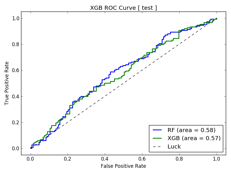
Depending upon the model parameters and the prediction date, the AUC of the ROC Curve will vary between 0.54 and 0.58. This model is barely passable, but we are getting a slight edge even with our basic data. We will need more game samples to have any confidence in our predictions.

After a model is created, we can run sflow in predict mode. Just specify the prediction date pdate, and SportFlow will make predictions for all cases in the predict.csv file on or after the specified date. Note that the predict.csv file is generated on the fly in predict mode and stored in the input directory.

Step 3: Now, let’s run SportFlow in predict mode, where all results will be stored in the output directory:

sflow --predict --pdate 2016-03-15

Conclusion Even with just one season of NCAA Men’s Basketball data, our model predicts between 52-54% accuracy. To attain better accuracy, we need more historical data vis a vis the number of games and other types of information such as individual player statistics. If you want to become a professional bettor, then you need at least 56% winners to break the bank.